Monte Carlo Methods to Simulate Stock Portfolio
Southern Methodist University
By Barry Daemi
Updated: May 12, 2023
$$\newcommand{\C}{\mathbb{C}} \newcommand{\R}{\mathbb{R}} \newcommand{\Z}{\mathbb{Z}} \newcommand{\Q}{\mathbb{Q}} \newcommand{\P}{\mathbb{P}}
\newcommand{\F}{\mathbb{F}} \newcommand{\N}{\mathbb{N}} \newcommand{\E}{\mathbb{E}}$$
1. Introduction
Quantitative finance is the meshing of computational mathematics and computational statistics with finance; the objective of this discipline is to analyze large financial datasets, so to derive meaningful insights and conclusions, and so to improve investment decisions and increased profitability. In this project we will cover the mathematical and statistical techniques required to simulated a stock portfolio in Python; the technical knowledge required for this project is some knowledge from Numerical Linear Algebra, Monte Carlo simulation, Multivariate statistics, alongside requiring some knowledge and proficiency in programming in Python.
In simulating a stock portfolio, we will be able to implement Value at Risk (VaR) and Conditional Value at Risk (CVaR), simulate option trading, and furthermore, improve said option trading schema with variance reduction techniques; the objective is to demonstrate a wide-breath of quantitative techniques, so to provide the reader with a large macro-view of the field. We hope that this project would prove to be a valuable online resource for the reader's asynchronous/synchronous studies in the field of Quantitative finance.
Note: Section 6. and 7. will be added in month or so from the publishing of this project on the portfolio website.
2. Stock Data Importation and Analysis
To begin, we imported the Python packages that would be utilized in this project, the following code block contains said packages: Pandas, Numpy, Matplotlib.pyplot, datetime, pandas_datareader, yfinance, seaborn and IPython. For the purpose of beautifying this Jupyter notebook custom CSS code was implemented through IPython.core.display's HTML package, and for that reason the following code block contains CSS code.
import random
import numpy as np
import pandas as pd
import scipy as sp
from scipy.stats import norm
import matplotlib.pyplot as plt
import datetime as dt
from pandas_datareader import data as pdr
import yfinance as yf
from yahoo_fin import options as op
import seaborn as sns
sns.set()
from IPython.core.display import HTML
HTML("""
<style>
ul.no-bullets {
  list-style-type: none;
  margin: 0;
  padding: 0;
}
table.GeneratedTable {
  width: 100%;
  background-color: #ffffff;
  border-collapse: collapse;
  border-width: 2px;
  border-color: #000000;
  border-style: solid;
  color: #000000;
}

table.GeneratedTable td, table.GeneratedTable th {
  border-width: 2px;
  border-color: #000000;
  border-style: solid;
  padding: 3px;
}

table.GeneratedTable thead {
  background-color: #3198ff;
}
</style>
""")
To import the stock data from Yahoo! Finance API (application programming interface), one has to utilize get_data_yahoo from pandas_datareader, which is an Python package that can interact with the Yahoo! Finance's API; the package is maintained by the Pandas development team. The passing arguments for get_data_yahoo is the stock's listing abbreviation (e.g. Microsoft stock's listing abbreviation is 'MSFT'), start Date and end Date; though it should be noted that the start date and end date need to be in datetime.datetime format, as this is the format that get_data_yahoo expects. To demonstrate the package functionality, we imported one year of Microsoft's stock data from time span of April 26, 2022 to May 12, 2023; the returned output is a pandas dataframe (e.g. pandas.core.frame.DataFrame) containing the aforementioned data.
endDate=dt.datetime.now();
startDate=endDate-dt.timedelta(days=381);
stockData=pdr.get_data_yahoo(['MSFT'],startDate,endDate)
stockData
[*********************100%***********************] 1 of 1 completed
| Open | High | Low | Close | Adj Close | Volume | |
|---|---|---|---|---|---|---|
| Date | ||||||
| 2022-04-27 | 282.100006 | 290.970001 | 279.160004 | 283.220001 | 280.468506 | 63477700 |
| 2022-04-28 | 285.190002 | 290.980011 | 281.459991 | 289.630005 | 286.816254 | 33646600 |
| 2022-04-29 | 288.609985 | 289.880005 | 276.500000 | 277.519989 | 274.823853 | 37073900 |
| 2022-05-02 | 277.709991 | 284.940002 | 276.220001 | 284.470001 | 281.706360 | 35151100 |
| 2022-05-03 | 283.959991 | 284.130005 | 280.149994 | 281.779999 | 279.042511 | 25978600 |
| ... | ... | ... | ... | ... | ... | ... |
| 2023-05-08 | 310.130005 | 310.200012 | 306.089996 | 308.649994 | 308.649994 | 21318600 |
| 2023-05-09 | 308.000000 | 310.040009 | 306.309998 | 307.000000 | 307.000000 | 21340800 |
| 2023-05-10 | 308.619995 | 313.000000 | 307.670013 | 312.309998 | 312.309998 | 30078000 |
| 2023-05-11 | 310.100006 | 311.119995 | 306.260010 | 310.109985 | 310.109985 | 31680200 |
| 2023-05-12 | 310.549988 | 310.440002 | 306.600189 | 308.970001 | 308.970001 | 19774696 |
263 rows × 6 columns
Above one can observe the imported Microsoft stock data; it only contains six column variables, 'Open': (e.g. opening price), 'Close': (e.g. closing price), 'High': (e.g. maximum price reached), 'Low': (e.g. minimum price reached), 'Adj Close': (e.g. Adjusted closing price after paying off the dividends) and 'Volume': (e.g. trading volume of that trading session).
Taking a granular perspective of the stock data, we can discern some level of insight on the stocks behavior and performance during this time span using basic data visualization and statistic techniques. As posed, let's first attain an illustrative perspective of the data; to do so, we had to reset the index of the stockData dataframe, so to capture the trading dates as a column variable named 'Date'; the printed result is found below.
stockDataModified=stockData;
stockDataModified.reset_index(inplace=True);
stockDataModified
| Date | Open | High | Low | Close | Adj Close | Volume | |
|---|---|---|---|---|---|---|---|
| 0 | 2022-04-27 | 282.100006 | 290.970001 | 279.160004 | 283.220001 | 280.468506 | 63477700 |
| 1 | 2022-04-28 | 285.190002 | 290.980011 | 281.459991 | 289.630005 | 286.816254 | 33646600 |
| 2 | 2022-04-29 | 288.609985 | 289.880005 | 276.500000 | 277.519989 | 274.823853 | 37073900 |
| 3 | 2022-05-02 | 277.709991 | 284.940002 | 276.220001 | 284.470001 | 281.706360 | 35151100 |
| 4 | 2022-05-03 | 283.959991 | 284.130005 | 280.149994 | 281.779999 | 279.042511 | 25978600 |
| ... | ... | ... | ... | ... | ... | ... | ... |
| 258 | 2023-05-08 | 310.130005 | 310.200012 | 306.089996 | 308.649994 | 308.649994 | 21318600 |
| 259 | 2023-05-09 | 308.000000 | 310.040009 | 306.309998 | 307.000000 | 307.000000 | 21340800 |
| 260 | 2023-05-10 | 308.619995 | 313.000000 | 307.670013 | 312.309998 | 312.309998 | 30078000 |
| 261 | 2023-05-11 | 310.100006 | 311.119995 | 306.260010 | 310.109985 | 310.109985 | 31680200 |
| 262 | 2023-05-12 | 310.549988 | 310.440002 | 306.600189 | 308.970001 | 308.970001 | 19774696 |
263 rows × 7 columns
With that completed, we were able to compose a script to plot the Microsoft stock price and traded volume for each trading session during the time span of April 26, 2022 to April 26, 2023.
plt.rc('figure',figsize=(15,13));

font={'family' : 'Times New Roman',
      'weight' : 'bold',
      'size'   : 22};
plt.rc('font',**font);

fig,axes=plt.subplots(2,1,gridspec_kw={'height_ratios':[3, 1.5]});
fig.tight_layout(pad=3);

date=stockData['Date']; close=stockData['Close'];
volume=stockData['Volume'];

plt.subplot(211);
plt.plot(date,close,color='red',linewidth=2,label='Price');
plt.xlabel('Date: Year-Month');
plt.ylabel('Stock Price');
plt.title('Microsoft Stock Analysis: April 26, 2022 to May 12, 2023');

plt.subplot(212);
plt.bar(date,volume,width=2,color='darkgrey');
plt.xlabel('Date: Year-Month');
plt.ylabel('Trading Volume');
plt.show();

These two illustrative plots are rather conventional, they serve the purpose of visualizing day-to-day price behavior/changes and daily trading activity of a stock. It is a rather simple technique to gain some useful sights on a stock daily behavior without having the need to implement any statistics and mathematics schema. A comparatively simple method approach to analyze, is the calculation of a stock's daily moving average and daily moving standard deviation. Particularly the moving standard deviation (MSTD) is a decent confirming indictor of market volatility. In example, a larger standard deviation means a larger spread and therefore a higher risk premium; while a smaller standard deviation means a lower spread and hence is associated with a lower risk premium. In regards to a moving standard deviation, the metric measures the spread between the closing price and moving average price; in the greater the spread, the higher the market volatility and risk premium.
To calculate the MSTD metric, one needs to first calculate the moving average (MA) metric, which is the following formulation:
$$\text{MA}=\frac{x_{1}+\cdots+x_{t}}{n} \tag{1}$$
where $x_{t} \in \R$ represents the price of the stock at given $t$ time, and hence $t$ represents a day in the time span between April 26, 2022 to April 26, 2023, e.g. $t \in [0,250]$, and $n$ represents the number of dates select from the time span. With ME calculated, we were then able to calculate the MSTD metric,
$$\text{MSTD}=\sqrt{\frac{\big(x_{1}-\text{MA}\big)^{2}+\big(x_{2}-\text{MA}\big)^{2}+\cdots+\big(x_{t}-\text{MA}\big)^{2}}{n}} \tag{2}$$
and similar to calculating a standard deviation measurement from the sample standard deviation formula (3), one only modification is needed to transform the equation from (3) to (2), replace the population mean, $\mu$, with the moving average (MA); derivation detail to MSTD can be found here [1].
To implement this derivation into Python, we choice to calculate the MA and MSTD for the daily percentage change in the stock daily instead of the daily price difference, as it was a more insightful/useful measurement of Microsoft stock's performance and volatility; specifically one can calculate a volatility measure with either simple returns or the logged returns, as evidenced in the script.
PercentChange=stockData['Close'].pct_change().dropna(); # percentage change in price; e.g. returns
RollingMean=PercentChange.rolling(3).mean().dropna(); # daily moving average
RollingSTD=PercentChange.rolling(3).std().dropna();   # daily standard deviation
AnnualVolatility=np.std(PercentChange)*np.sqrt(252);  # annualized volatility by simple returns

a=stockData['Close'];
r=[np.log(a[i+1]/a[i]) for i in range(len(a)-1)];
r=pd.Series(np.array(r));                             # Log-Returns
RollingMean2=r.rolling(3).mean().dropna();
RollingSTD2=r.rolling(3).std().dropna();
AnnualVolatility2=np.std(r)*np.sqrt(252);

print("Expected Average Return: " + str(np.mean(PercentChange)))
print("Standard deviation of Returns: " + str(np.std(PercentChange)))
print(" ")
print("STD of simple returns: " + " "*35 + "STD of Log Return:")
print("Annual Volatility: " + str(AnnualVolatility) + " "*22 + "Annual Volatility: " + str(AnnualVolatility2));
print("Monthly Volatility: " + str(AnnualVolatility/np.sqrt(12)) + " "*19 + "Monthly Volatility: "
      + str(AnnualVolatility2/np.sqrt(12)));
print("Weekly Volatility: " + str(AnnualVolatility/np.sqrt(52)) + " "*20 + "Weekly Volatility: "
      + str(AnnualVolatility2/np.sqrt(52)));
print("Daily Volatility: " + str(np.std(PercentChange)) + " "*21 + "Daily Volatility: " + str(np.std(r)) );


plt.rc('figure',figsize=(15,13));

font={'family' : 'Times New Roman',
      'weight' : 'bold',
      'size'   : 22};
plt.rc('font',**font);

fig,axes=plt.subplots(2,1,gridspec_kw={'height_ratios':[2, 2]});
fig.tight_layout(pad=3);

plt.subplot(211);
plt.bar(date[3:len(a)],RollingMean,width=1.5,color='darkgrey')
plt.xlabel('Date: Year-Month');
plt.ylabel('Daily Moving Average');
plt.title('Microsoft Stock Analysis: April 26, 2022 to May 12, 2023');

plt.subplot(212);
plt.bar(date[3:len(a)],RollingSTD,width=1.5,color='darkgrey')
plt.xlabel('Date: Year-Month');
plt.ylabel('Daily Moving Standard Deviation');
plt.show();
Expected Average Return: 0.0005614932289200549
Standard deviation of Returns: 0.02144256450318899

STD of simple returns:                                    STD of Log Return:
Annual Volatility: 0.34039015888139595                      Annual Volatility: 0.33975104162617137
Monthly Volatility: 0.09826217492983673                   Monthly Volatility: 0.0980776776701629
Weekly Volatility: 0.04720362198116181                    Weekly Volatility: 0.04711499236444081
Daily Volatility: 0.02144256450318899                     Daily Volatility: 0.021402303900428646

To compare the daily volatility measurement against the stock performance during the time span; the following script plots the two cartesian plots along one another, for an easy comparison. An signicant observation is that a volatility measure spikes during dramatic changes to the stock price, and falls during steady increases or decreases in the stock price. Consequentially a historical volatility metric can only effectively measure dramatic shifts in the market, it cannot measure the long-run trend of a market, or capture the type of price shift, either positive or negative, instead it can only measure the risk-level and magnitude of the shift.
plt.rc('figure',figsize=(15,13));

font={'family' : 'Times New Roman',
      'weight' : 'bold',
      'size'   : 22};
plt.rc('font',**font);

fig,axes=plt.subplots(2,1,gridspec_kw={'height_ratios':[2, 2]});
fig.tight_layout(pad=3);

plt.subplot(211);
plt.plot(date,close,color='red',linewidth=2,label='Price');
plt.xlabel('Date: Year-Month');
plt.ylabel('Stock Price');
plt.title('Microsoft Stock Analysis: April 26, 2022 to May 12, 2023');

plt.subplot(212);
vol=RollingSTD/np.sqrt(52);
vol2=RollingSTD2/np.sqrt(52);
plt.plot(date[3:len(date)],vol,color='red',linewidth=1.5,label='Simple Returns');
plt.plot(date[3:len(date)],vol2,color='blue',linewidth=1.5,label='Logged-Returns');
plt.xlabel('Date: Year-Month');
plt.ylabel("Daily Volatility")
plt.title('Microsoft Stock Analysis: April 26, 2022 to May 12, 2023');
plt.legend();
plt.show()

A better votalitity metric to discern market sentiment over an entire stock exchange (e.g. S&P 500 Index) is the Volatility Index (VIX), which was created by Chicago Board of Options Exchange. This volatility metric measures the level of volatility that an stock exchange will experience over the next 30 days; the measurement can be used to discern the overal sentiment of the market; i.e. when VIX is high, the market is likely in a up-swing and it is time to buy; while VIX is low, it is likely the market is overpriced, and it is time to sell.
A more specific measurement of single security votatility is the Implied Volatility (IV) metric, which is calculated solely upon the current market value of that specific single security's put/call options. The most conventional approach to attain the current price of the security's put/call option is executing a Black-Scholes option pricing model to attain a theoretical estimate for one of the options; but as no close form solution exist for the implied volatility measurement, one needs to estimate it; there exist different schema, such as, beta coefficients, option pricing models (e.g. Iterative search), and standard deviations of returns, but the simplest and most practical is Iterative search.
Digressing the implied volatility metric is similar to the historical volatility matric, as both of these measurements can capture the realize variation in the stock price (not when implied volatility is the lone measurement); but cannot capture the ovaral sentiment of the market, or disginuish the type of variation. Instead one conventionally calculates both of these metrics to compared them against one another, to guage the risk-premium in the market. If both metric indicate similar volatility, then the option price is considered fair, and no possible price deviation away from this price equilibrium exists to advantage of. When these metrics deviate, then that means the option is either overvalued or undervalued, and therefore, a strategy exists that can be taken advantage of, that can generate a proift.
Digressing another angle of analysis is the analyzing of the distribution of returns a financial instrument/product generates; different financial instruments/products generate different types of distribution with different statistical characteristics (e.g. center, spread, skewedness, et ceteria). Nevertheless unlike most other financial instrument, securities (e.g. stocks) are assumed to possess gaussian distributed returns. Conventionally outside the influence of a "Black swan" event or a "White swan" event, the price change and percentage price change (e.g. rate-of-return) of a security will both possess a gaussian shaped distribution with skewed fat tails, due to outliers. Due to these outlier returns, the shape of a pseudo-gaussian distribution that cannot be properly mapped by the gaussian function,
$$ f(x) = \frac{1}{\sigma \sqrt{2 \pi}}\text{exp}\bigg(-\frac{1}{2}\big(\frac{x-\mu}{\sigma}\big)^{2}\bigg) \tag{3}$$
and so, the returns possesses a mix-distribution shape, and thus, is defined by a undefined closed formed mix-density function, or is defined by a mix-density function with no close form solution. The most plausible explanation is that the return distribution is a type of mixed gaussian distribution, with a mix-gaussian density function; this claims is from Yan and Han (2019): [2].
To demonstrate the mix-gaussian nature of stock returns, we generated a histogram plot with the price changes that occur during the time span from April 26, 2022 to May 01, 2023, and subsequently plotted the corresponding theoretical gaussian function that said sampling formed. To test the normality of the sampling's distribution, a Jarque-Bera goodness of fit test [3] and Shapiro-Wilk Test [4] were performed and there subsequent hypotheses tested conducted [5].
# Calculate the price changes over the time span
price=stockDataModified['Close'];
price_diff=[price[i+1]-price[i] for i in range(len(price)-1)];

# Tests the normality of the price changes with Jarque-Bera test
print("To test the normality of the rate-of-return distribution of Microsoft stock:");
print(" ");
print("Jarque-Bera goodness of fit test: " + str(sp.stats.jarque_bera(stockDataModified['Close'])));
print(" ");
print("Shapiro-Wilk Test: " + str(sp.stats.shapiro(stockDataModified['Close'])));
print(" ");
print("Mean: " + str(np.mean(price_diff)) + " "*10 + "Standard deviation: " + str(np.std(price_diff)));

x_axis=np.linspace(min(price_diff),max(price_diff),len(price_diff));
mean=np.mean(price_diff); std=np.std(price_diff);

plt.rc('figure',figsize=(8,6));

fig,ax = plt.subplots();
temp = ax.hist(price_diff,100,density=True);
plt.plot(x_axis,norm.pdf(x_axis,mean,std));
plt.xlabel("Price change");
plt.ylabel("Probability");
plt.title("Distribution of Price Change - Microsoft Stock: April 26, 2022 to May 12, 2023");
plt.show();
To test the normality of the rate-of-return distribution of Microsoft stock:

Jarque-Bera goodness of fit test: SignificanceResult(statistic=9.41195194561631, pvalue=0.009041086056433497)

Shapiro-Wilk Test: ShapiroResult(statistic=0.9769615530967712, pvalue=0.0002916510566137731)

Mean: 0.0982824427480916          Standard deviation: 5.473574931430873

Result was a distribution with a closely gaussian shaped; it was center at a mean of $0.139$ USD and dispersed with a standard deviation of $5.593$ USD. And aforementioned the sample distribution possessed outliers that enlarged the tails of the distribution. To test the normality of the sampled distribution, a Jarque-Bera test was administed with the following hypotheses and an $\alpha=0.05$:
| Jarque–Bera test | |
|---|---|
| Null Hypothesis ($H_{0}$): | Skewness is zero and the excess kurtosis is zero. |
| Alternative Hypothesis ($H_{a}$): | Skewness is greater than zero and also excess kurtosis is greater than zero. |
Jarque-Bera test was implemented through jarque_bera() from the statistical package from Scipy; the result was a chi-square statistic of $6.691$, which has a p-value of $0.0352$. With testing our hypotheses, $\alpha = 0.05 > \text{p-value} = 0.0352$, which means we reject the null hypothesis, and therefore the sample distribution possesses a skewness and excess kurtosis that is greater than zero and hence means that the stock returns is not a standard normally distributed random variable.
Are the samples from a normally distributed population? With Shapiro-Wilk test that question can be statistically tested for, and with the following hypotheses we administered aforementioned statistical test with an $\alpha=0.05$:
| Shapiro–Wilk test | |
|---|---|
| Null Hypothesis ($H_{0}$): | Sample originate from a normally distributed population. |
| Alternative Hypothesis ($H_{a}$): | Sample originate from a non-gaussian distributed population. |
To implement Shapiro–Wilk test the shapiro() function from the statistical package from Scipy was used; the output was a test statistic of $0.983$, which has a p-value of $0.00445$; hypothesis testing, $\alpha=0.05 > \text{p-value}=0.00445$ and therefore we must reject the null hypothesis in favor of the alternative hypothesis, and hence, the samples originate from a non-gaussian distribution population.
Changing the sample random variable to percentage change in the price, does not change the type of distribution that is manifested, the sample distribution is still a mixed-gaussian random variable with a mix-gaussian density,
$$f(X_{i}|\Theta)=\sum_{k=1}^{K} \omega_{k} \frac{1}{\big(2 \pi\big)^{d/2}\big(\det\big(\Sigma_{k}\big)\big)^{1/2}}, \tag{4}$$
where $X_{i}=\big[ x_{i}, y_{i}, \ldots \big]$ for,
$$\text{exp}\bigg( -\frac{1}{2} \big( X_{i} - \mu_{k} \big)^{T} \Sigma_{k}^{-1} \big( X_{i} - \mu_{k} \big) \bigg), \tag{5}$$
with $i=1,2,\ldots, n$; $\omega_{k}$ (with $k=1,2,\ldots,K$) denotes the weight for each of the components with a restrictive condition that $\sum_{k=1}^{K} \omega_{k}=1$ [2]. The same two statistical tests for normallity were administered for this new sampled random variable, both with an $\alpha = 0.05$.
PercentP=stockDataModified['Close'].pct_change().dropna(); # percentage change of the stock price

print("To test the normality of the percentage rate-of-return distribution of Microsoft stock:");
print(" ");
print(sp.stats.jarque_bera(PercentP));
print(" ");
print("Shapiro-Wilk Test: " + str(sp.stats.shapiro(PercentP)));
print(" ");
print("Mean: " + str(np.mean(PercentP)) + " "*10 + "Standard deviation: " + str(np.std(PercentP)));


x_axis=np.linspace(min(PercentP),max(PercentP),len(PercentP));
mean=np.mean(PercentP); std=np.std(PercentP);

plt.rc('figure',figsize=(8,6));

fig,ax = plt.subplots();
temp = ax.hist(PercentP,50,density=True);
plt.plot(x_axis,norm.pdf(x_axis,mean,std));
plt.xlabel("Rate-of-returns");
plt.ylabel("Frequency");
plt.title("Distribution of % Price Change - Microsoft Stock: April 26, 2022 to May 12, 2023");
plt.show();
To test the normality of the percentage rate-of-return distribution of Microsoft stock:

SignificanceResult(statistic=23.24002860265311, pvalue=8.984458547888842e-06)

Shapiro-Wilk Test: ShapiroResult(statistic=0.9830119013786316, pvalue=0.0032606280874460936)

Mean: 0.0005614932289200549          Standard deviation: 0.02144256450318899

For the Jarque–Bera test results, the chi-square statistic was $18.150$, which has a p-value of $0.000114$; hence, $\alpha = 0.05 > \text{p-value} = 0.000114$, which means we reject the null hypothesis, the sampled distribution possesses a skewness and excesss kurtosis greater than zero. Subsequently, the Shapiro–Wilk test resulted with a test statistic $0.985$ with a p-value of $0.00799$; hypothesis testing, $\alpha=0.05 > \text{p-value} = 0.00799$, and therefore, we reject the null hypothesis yet again, and hence the samples are not from a gaussian shaped distribution.
3. Simulate a Stock Portfolio
In this section, we will cover the material needed to actually simulate a Stock portfolio, given the assumption that there are no "black swan" or "white swan" events in the given time span, $[$startDate,endDate$]$, and therefore for simplification we assumed that each of the rate-of-returns random variables are gaussian distributed, $\mathcal{N}(\mu, \sigma^{2})_{i}$, $i=1,2,\ldots,n$. In addition, given that this simulated Stock portfolio will contain multiple stocks (e.g. $i=1,2,\ldots,n$), the collection of returns from this mix portfolio will be modeled by a multivariate normal random variable, $\mathcal{N}(\vec{\mu},\Sigma)$, where $\vec{\mu}$ is the mean vector and $\Sigma$ the covariance matrix.
To generate this correlated multivariate gaussian random variable, we used the cholesky decomposition of the covariance matrix approach [6,7], and to generate the standard gaussian random variables that makeup the foundation of this correlated multivariate gaussian random variable scheme - we used Marsaglia's polar method to generate standard standard normal random variables, $\mathcal{N}(\mu,\sigma^{2})$. To begin, Marsaglia's polar method [8] is an modified Box-Muller algorithms [9] that avoids the cost of computating the (computationally) expensive trigonometric functions in the previous aforementioned pseduo-random number (PRN) sampling algorithm, and therefore is a more computationally efficient PRN sampling algorithm. Nonetheless the Box-Muller transform PRN formulas,
$$Z_{1}=R\cos{\Theta}=\sqrt{-2\ln\big(U_{1}\big)}\cos\big(2\pi U_{2}\big), \tag{6}$$
$$Z_{2}=R\sin{\Theta}=\sqrt{-2\ln\big(U_{1}\big)}\sin\big(2\pi U_{2}\big), \tag{7}$$
where $U_{1},U_{2} \in U[0,1]$ are two uniform distributed random variables, and the radius is defined by $R=\sqrt{-2\ln(U_{1})}$ and the angle is defined by $\Theta = 2\pi U_{2}$. In essence the the Box-Muller PRN method transforms squared-cartesian coordinates to round polar coordinates within the bounds of the unit circle. Marsaglia's polar PRN algorithm avoid the trigonometric function, by replacing the angle formula with,
$$\Theta_{X}=\frac{W_{1}}{\sqrt{W_{1}^{2}+W_{2}^{2}}}, \tag{8}$$
$$\Theta_{Y}=\frac{W_{2}}{\sqrt{W_{1}^{2}+W_{2}^{2}}}, \tag{9}$$
where $\Theta_{X}$ represent the angle for the x-coordinate (on the unit cirle), and $\Theta_{Y}$ represents the angle for the y-coordinate (on the unit cirle).
Proceeding with the implementation of Marsaglia polar method, despite being an transformation method, we had to take a reject-acceptance methodology to generation process, so to be able to attain the desired standard normal random variable. Specifically as each pseudo-random sample must be conditionally test against $W_{1}^{2}+W_{2}^{2} < 1$, only a single pseudo-random sample was generated at each iteration of the PRN schema. In addition as the uniformed random variables for Marsaglia polar method are suppose to be $U[-1,1]$ instead of $U[0,1]$, we used $U[-1,1]= 2 \cdot U[0,1] - 1$ to transform the unfirom random variables from $U[0,1]$ to $U[-1,1]$, which is necessary as the uniform samples must encompass the entire unit circle. Combining the Box-Muller transform with the Marsaglia modifications, results in the following formulation:
$$X_{1}=W_{1}\sqrt{\frac{-2\ln\big(W_{1}^{2}+W_{2}^{2}\big)}{W_{1}^{2}+W_{2}^{2}}}, \tag{10}$$
$$X_{2}=W_{2}\sqrt{\frac{-2\ln\big(W_{1}^{2}+W_{2}^{2}\big)}{W_{1}^{2}+W_{2}^{2}}}. \tag{11}$$
With the derivation complete for Marsaglia’s Polar Method, it was rather simple to compose a Python script for the PRN sample algorithm. As aforementioned the script took an acceptance-rejection approach to sampling, and so, an iter and while loop method was implemented. Upon execution of the following algorithm an standard normal random variable, $\mathcal{N}(\mu,\sigma^{2})$ with $n$ size is generated [10]; with that, the next step to generate a specific correlated multivariate gaussian random variable is the derivation and implementation of Cholesky decomposition.
def polar_method(n):
    i=0;
    output=np.zeros(n);
    while i < n:
        U1=np.random.uniform(0,1,1); U2=np.random.uniform(0,1,1);
        W1=2*U1-1; W2=2*U2-1;
        if (W1**2+W2**2) < 1:
            output[i]=W1*np.sqrt(-2*np.log(W1**2+W2**2)/(W1**2+W2**2));
            i=i+1;
    return output;
A linear system is a collection of linear equations that can take the shape as a linear system of equations, or as an augmented matrix form:
$$\begin{array}{ccc} a_{1,1} x_{1}+\cdots+a_{1,m} x_{n} & = & b_{1} \\ \vdots & \vdots & \vdots \\ a_{n,1} x_{1}+\cdots+a_{n,m} x_{n} & = & b_{n} \end{array} \to \begin{bmatrix} a_{1,1} & \cdots & a_{1,m} \\ \vdots & \ddots & \vdots \\ a_{n,1} & \cdots & a_{n,m} \end{bmatrix} \left[ \begin{array}{c} x_{1} \\ \vdots \\ x_{n} \end{array} \right] = \left[ \begin{array}{c} b_{1} \\ \vdots \\ b_{m} \end{array} \right]. \tag{12}$$
A linear system is conventionally denoted as $\text{Ax}=\text{b}$, where matrix $\text{A}$ is a linear mapping function between $\R^{n}$ and $\R^{m}$: e.g., $\text{A}: \R^{n} \to \R^{m}$ where $x \in \R^{n}$ and $b \in \R^{m}$ [11]. To solve the linear system, it has to be at least reduced to upper triangular form:
$$\begin{bmatrix} \widetilde{a}_{1,1} & \widetilde{a}_{1,2} & \cdots & \widetilde{a}_{1,m} \\ 0 & \widetilde{a}_{2,2} & \cdots & \widetilde{a}_{2,m}\\ \vdots & 0 & \ddots & \vdots \\ \vdots & \vdots \\0 & 0 & \cdots & \widetilde{a}_{n,m} \end{bmatrix} \left[ \begin{array}{c} x_{1} \\ \vdots \\ x_{b} \end{array} \right] = \left[ \begin{array}{c} \widetilde{b}_{1} \\ \vdots \\ \widetilde{b}_{m} \end{array} \right], \tag{13}$$
this can be accomplished through Gaussian elimination [12]; from here backward substitution can be implemented to solve for each of the $x_{i}$, from descending order, $i=n, n-1, n-2, \ldots, 1$. A step could be taken further, instead of reducing matrix $\text{A}$ to upper triangular form, what happens if it were to be reduced to row-reduced echelon form:
$$\begin{bmatrix} 1 & 0 & \cdots & 0 \\ 0 & 1 & \cdots & 0 \\ \vdots & 0 & \ddots & \vdots \\ \vdots & \vdots \\0 & 0 & \cdots & 1 \end{bmatrix} \left[ \begin{array}{c} x_{1} \\ \vdots \\ x_{b} \end{array} \right] = \left[ \begin{array}{c} \widetilde{b}_{1} \\ \vdots \\ \widetilde{b}_{m} \end{array} \right], \tag{14}$$
in this form the target vector, $\widetilde{b}$, becomes the solution vector, $\overrightarrow{x}$; e.g. $\overrightarrow{x}=\widetilde{b}$, where $\overrightarrow{x} \in \R^{n}$ and $\widetilde{b} \in \R^{m}$, and lastly, as matrix $\text{A}$ must be full-rank to possess an unique solution $\overrightarrow{x}$, the dimensions of both fields must agree $n=m$. Otherwise, when matrix $A$ is rank-deficient, $n \neq m$, then the linear system is either over-determined (more equations than unknown variables) or under-determined (more unknown variables than equations), and therefore, $Ax \neq b$, are not equal and hence no solution exists for this linear system, but for a non-unique least squares solution, $\hat{x}$, which can be attained through the ordinary least squares algorithm (e.g. Ordinary Least Squares regression (e.g., Linear regression).
The algorithmic form of Gaussian elimination is LU decomposition [13,14], where matrix $\text{A}$ is decomposed into $\text{L}\text{U}=\text{A}$, given that $\text{U}$ is the upper triangular form of matrix $\text{A}$ and that $\text{L}$ is composed of the gaussian elimination operations that transformed matrix $\text{A}$ into upper triangular form, $\text{U}$. To construct matrix $\text{L}$, all of the elimination matrices must be accumulated, as such,
$$\text{L}_{m-1}\text{L}_{m-2}\cdots \text{L}_{2}\text{L}_{1}\text{A}=\text{U} \to \text{A}=\text{L}\text{U} \; \; \text{where} \; \; \text{L}=\text{L}_{1}^{-1}\text{L}_{2}^{-1}\cdots \text{L}_{m-2}^{-1}\text{L}_{m-1}^{-1}, \tag{15}$$
and given that elimination matrices take the form,
$$\text{L}_{k}= \begin{bmatrix} 1 & & & & \\ & \ddots & & & \\ & & 1 & \\ & & -l_{k+1,k} & 1 & \\ & & \vdots & & \ddots & \\ & & -l_{m,k} & & & 1 \end{bmatrix}=\prod_{j=k+1}^{m} E_{a}(k,j,-l_{j,k}), \tag{16}$$
where the multiplers $l_{j,k}=\frac{x_{j,k}}{x_{k,k}}$. And therefore with the accumulation of elimination matrices through inverse-and-matrix-multiplication forms the lower triangular matrix $\text{L}$:
$$\text{L}=\text{L}_{1}^{-1}\text{L}_{2}^{-1}\cdots\text{L}_{m-2}^{-1}\text{L}_{m-1}^{-1}=\begin{bmatrix} 1 & & & & \\ l_{2,1} & 1 & & & \\ l_{3,1} & l_{3,2} & 1 & \\ \vdots & \vdots & \ddots & \ddots & \\ l_{m,1} & l_{m,2} & \cdots & l_{m,m-1} & 1 \end{bmatrix}. \tag{17}$$
Applying the inverse matrix $\text{L}$ to matrix $\text{A}$ gives matrix $\text{U}$, e.g. $\text{L}^{-1}\text{A}=\text{U}$. A pseudio-code example of LU decomposition is as followed:
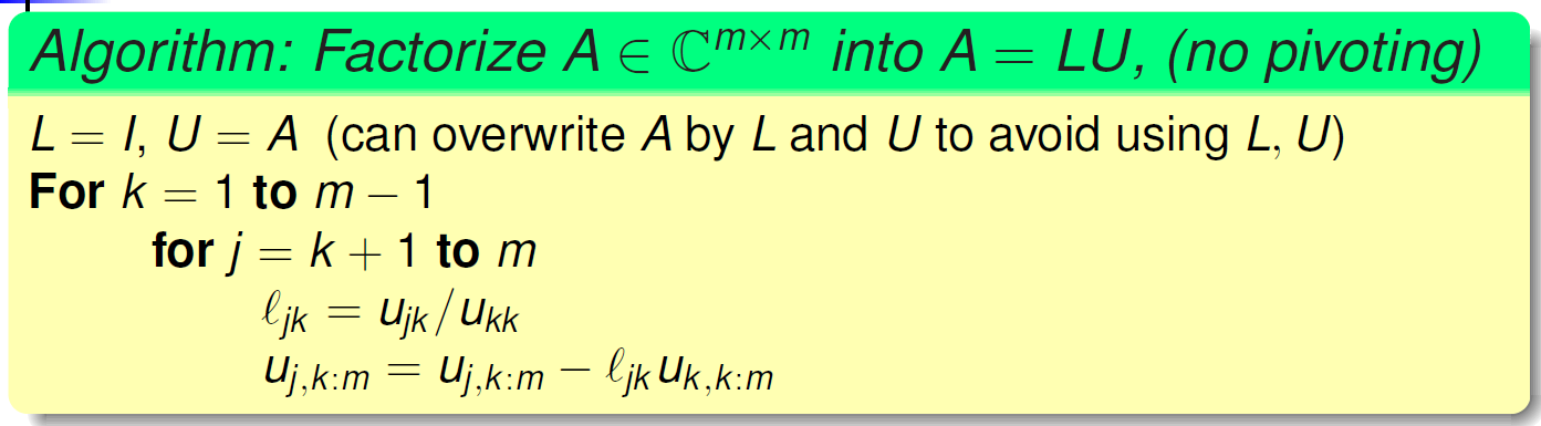
Coming full cirle, solving the linear system, $\text{A}\text{x}=\text{b}$ with LU decomposition at the matrix-level is as attributed below:
$$\text{A}\text{x}=\text{b} \to \text{LU}\text{x}=\text{b} \to \text{L}^{-1}\text{LU}\text{x}=\text{L}^{-1}\text{b} \to \text{U}\text{x}=\text{L}^{-1}\text{b} \to \text{U}\text{x}=\text{y}, \tag{18}$$
where $\text{y}=\text{L}^{-1}\text{b}$. An astute observation would be to recognize that $\text{U}\text{x}=y$ is equation (13), and that the LU decomposition algorithm arrived to the same upper triangular form as non-automated gaussian elimination.
Cholesky decomposition is an special variation of the LU decomposition algorithm, though due to the variation in the algorithm structure/approach, the Cholesky fractorization algorithm can only handle symmetric-positive-definite (SPD) and Hermitian-positive-definite (HPD) matrices. The elimination equations for Cholesky factorization is,
$$\text{L}_{j,j}=\pm\sqrt{a_{j,j}-\sum_{k=1}^{j-1}\text{L}_{j,k}\text{L}_{j,k}^{*}}, \tag{19}$$
$$\text{L}_{i,j}=\frac{1}{\text{L}_{i,j}}\bigg( a_{i,j} - \sum_{k=1}^{j-1} \text{L}_{i,k}\text{L}_{j,k}^{*}\bigg) \;\;\; \text{for} \; i > j. \tag{20}$$
With that derivation completed, one can compose the Python implementation of Cholesky factorization; which is done in the code block following this sentence.
def cholesky_decomposition(M):
    A=np.copy(M); m,n=A.shape;
    R=np.zeros((m,n));

    for k in range(n):
        R[k,k]=np.sqrt(A[k,k]);
        R[k,k+1:]=A[k,k+1:]/R[k,k];
        for j in range(k+1,n):
            A[j,j:]=A[j,j:]-R[k,j]*R[k,j:];
    return R.T;
To generate the correlated multivariate gaussian random variable, the covariance matric, $\Sigma$, must be SPD and HPD, which means it is a squared matrix of size $n$ x $n$. The aforementioned covariance matrix $\Sigma$ is decomposed by Cholesky factorization, the resulting Cholesky factor, $\text{L}$, is subsequentially matrix-multiplied with a standard normal random variable of size $n$ x $m$. For an example, suppose there exists a $2$ x $2$ covariance matrix,
$$\Sigma=\begin{bmatrix} \Sigma_{1,1} & \Sigma_{1,2} \\ \Sigma_{2,1} & \Sigma_{2,2} \end{bmatrix} = \begin{bmatrix} \sigma_{1}^{2} & \sigma_{1}\sigma_{2}\rho \\ \sigma_{1}\sigma_{2}\rho & \sigma_{2}^{2} \end{bmatrix} \tag{21}$$
and that a Cholesky decomposition was performed upon it; the resulting computation would follow, let $\alpha=\sqrt{\Sigma_{1,1}}$, and so,
$$\Sigma=\begin{bmatrix} \Sigma_{1,1} & \Sigma_{1,2} \\ \Sigma_{2,1} & \Sigma_{2,2} \end{bmatrix} = \begin{bmatrix} \alpha & 0 \\ \frac{\Sigma_{2,1}}{\alpha} & \sqrt{\Sigma_{2,2}-\bigg( \frac{\Sigma_{2,1}}{\alpha} \bigg)^{2}} \end{bmatrix} \begin{bmatrix} \alpha & \frac{\Sigma_{2,1}}{\alpha} \\ 0 & \sqrt{\Sigma_{2,2}-\bigg( \frac{\Sigma_{2,1}}{\alpha} \bigg)^{2}} \end{bmatrix} = \text{L}\text{L}^{T}. \tag{22}$$
Replacing the abritary $\Sigma_{i,j}$ (e.g. $i=1,2$, $j=1,2$) with the theoretical values of a conventional covariance matrix, we attain,
$$L= \begin{bmatrix} \alpha & 0 \\ \frac{\Sigma_{2,1}}{\alpha} & \sqrt{\Sigma_{2,2}-\bigg( \frac{\Sigma_{2,1}}{\alpha} \bigg)^{2}} \end{bmatrix} = \begin{bmatrix} \sqrt{\sigma_{1}^{2}} & 0 \\ \frac{\sigma_{1}\sigma_{2}\rho}{\sqrt{\sigma_{1}^{2}} } & \sqrt{\sigma_{2}^{2}-\bigg( \frac{\sigma_{1}\sigma_{2}\rho}{\sqrt{\sigma_{1}^{2}} } \bigg)^{2}} \end{bmatrix}=\begin{bmatrix} \sigma_{1} & 0 \\ \sigma_{2}\rho & \sigma_{2}\sqrt{1-\rho^{2}} \end{bmatrix}. \tag{23}$$
With the Cholesky factor $\text{L}$, suppose there exists a multivariate standard normal, $\text{Z}=\mathcal{N}\bigg(\overrightarrow{\mu}= \left[ \begin{array}{c} 0 \\ 0 \end{array} \right] , \Sigma= \begin{bmatrix} 1 & 0 \\ 0 & 1 \end{bmatrix} \bigg)$ of size $2$ x $m$; computing the inner product of these two matrices generates the corresponding correlated multivariate normal random variable, $X=\mathcal{N}(\overrightarrow{\mu},\Sigma)$:
$$\text{Z}=\mathcal{N}\bigg(\overrightarrow{\mu}= \left[ \begin{array}{c} 0 \\ 0 \end{array} \right] , \Sigma= \begin{bmatrix} 1 & 0 \\ 0 & 1 \end{bmatrix} \bigg)=\begin{bmatrix} z_{1,1} & \cdots & z_{1,m} \\ z_{2,1} & \cdots & z_{2,m} \end{bmatrix}, \tag{24}$$
$$X=\text{L}^{T}\text{Z}=\begin{bmatrix} \sigma_{1} & \sigma_{2}\rho \\ 0 & \sigma_{2}\sqrt{1-\rho^{2}} \end{bmatrix} \begin{bmatrix} z_{1,1} & \cdots & z_{1,m} \\ z_{2,1} & \cdots & z_{2,m} \end{bmatrix}=\begin{bmatrix} \sigma_{1} \cdot z_{1,1} + \sigma_{2}\rho \cdot z_{2,1} & \cdots & \sigma_{1} \cdot z_{1,m} + \sigma_{2}\rho \cdot z_{2,m} \\ \sigma_{2}\sqrt{1-\rho^{2}} \cdot z_{2,1} & \cdots & \sigma_{2}\sqrt{1-\rho^{2}} \cdot z_{2,m} \end{bmatrix}. \tag{25}$$
For a correlated multivariate gaussian random variable to model the theoretical returns of a specific stock portfolio, the stock portfolio covariance matrix, $\Sigma$, must be computated alongside the average return for each of the stocks, $\overrightarrow{\mu}$. For equation (25) to model the theoretical returns of a specific stock portfolio, one additional modification is needed,
$$\text{Returns}=\overrightarrow{\mu} + X = \overrightarrow{\mu}+\begin{bmatrix} \sigma_{1} \cdot z_{1,1} + \sigma_{2}\rho \cdot z_{2,1} & \cdots & \sigma_{1} \cdot z_{1,m} + \sigma_{2}\rho \cdot z_{2,m} \\ \sigma_{2}\sqrt{1-\rho^{2}} \cdot z_{2,1} & \cdots & \sigma_{2}\sqrt{1-\rho^{2}} \cdot z_{2,m} \end{bmatrix}, \tag{26}$$
as the spread of the returns distribution was captured through the Cholesky factor, $\text{L}$, the center shift needs to be captured as well, so to center the correlated multivariate random variable at the correct center point, $\overrightarrow{\mu}$ is added to equation (25) to shift the center to the corrent center point.
With the technique to generate theoretical returns completely explain; we must proceed onto to how to generate a simulated stock portfolio; to do so, one must import real-stock data for each of the stock that makeup the composition of the simulated portfolio. In our simulated stock portfolio, we chose to invest into Microsoft and Apple stocks during the time span, $[$startDate,endDate$]$, then decided the portfolio diversification on a random weight formula, weights/=np.sum(weights);. A more sophisticated and robust approach to determining portfolio diversification is Von Neumann-Morgenstern Portfolio Theory (or Expected Utility Approach Portfoio Theory), which is a risk mitigation schema through utility approach, which can estimate the perfect weights for a given stock portfoio; e.g. it can provide the proportions to a perfectly diversified portfolio.
A significant draw back with Von Neumann-Morgenstern Portfolio Theory, is that it is only applicable to stock portfolio of two types: Portfolio #1: one riskless asset (i.e. government bond/commercial paper) and risky asset (i.e. risky financial instrument) and Portfolio #2: two risky assets. If a stock portfolio exceeds two assets, then Von Neumann-Morgenstern Portfolio Theory fails to be applicable, as it lack the mathematical framework to handle this scenario; though we have a proposed solution to this problem, though we will leave that inquiry for another project, as it is too lengthy to address here. Nonetheless, if given the choice our simulated stock portfolio consisted of two risky assets (i.e. our case securities), and so, Von Neumann-Morgenstern Portfolio Theory is a valid risk mitigation/diversification schema. On another hand, if one desire to maximize return while mitigating risk (mimimizing variance), then one would choose Markowitz Mean-Variance Portfolio Theory (or Mean-Variance Portfolio theory, or Modern Portfolio Theory) [15,16].
To retrieve the stock data from Yahoo! Finance API, the following Python function was written, which retrieved said stock data for the specified stocks (e.g. stocklist=[]); as the aim is to simulate daily returns for each of the stocks, the mean vector and covariance matrix were computed and returned.
def get_data(stocks,start,end):
    stockData=pdr.get_data_yahoo(stocks,start,end);
    stockData=stockData['Close']
    returns=stockData.pct_change().dropna();
    meanReturnsVector=returns.mean();
    covMatrix=returns.cov();
    return returns,meanReturnsVector, covMatrix;
It was chosen that the simulated stock portfolio be composed of Microsoft ("MSFT") and Apple Inc. ("AAPL"); to retrieve the stock data for Microsoft and Apple Inc., a list ticker names, stockList=['MSFT','AAPL'], were passed through get_data(); additionally, the stock data that was retrieved covered the past 1,825 day period (or the last 5 years): May 11, 2018 to May 10, 2023. To display the mean vector and covariance matrix, it was printed to console for reader convenience; from the time of the creation of this project,
$$\overrightarrow{\mu}=\left[ \begin{array}{c} 0.001250 \\ 0.001104 \end{array} \right] \;\;\; \text{and} \;\;\; \text{Cov(x)}= \begin{bmatrix} 0.000441 & 0.000315 \\ 0.000315 & 0.000384 \end{bmatrix}, \tag{27}$$
where the covariance was determined by determinant, $| \text{Cov(x)} | > 0$, to be Positive-Definite and symmetrical through observation.
stockList=['MSFT','AAPL'];
endDate=dt.datetime.now(); startDate=endDate-dt.timedelta(days=1825);
Returns,meanReturnsVector,covMatrix=get_data(stockList,startDate,endDate);
weights=np.random.random(len(meanReturnsVector));
weights/=np.sum(weights);
print("Mean  Returns Vector: \n" + str(meanReturnsVector));
print(" ");
print("Covariance matrix: \n" + str(covMatrix));
print(" ");
print("Determinant: Det(covMatrix) =" + str(np.linalg.det(covMatrix)));
print(" ");
print("Portfolio Asset distribution: " + str(weights));
[*********************100%***********************]  2 of 2 completed
Mean  Returns Vector:
AAPL    0.001254
MSFT    0.001105
dtype: float64

Covariance matrix:
          AAPL      MSFT
AAPL  0.000440  0.000315
MSFT  0.000315  0.000383

Determinant: Det(covMatrix) =6.977306935631813e-08

Portfolio Asset distribution: [0.81337678 0.18662322]
The following is a simulation of the performance of 100 theoretical stock portfolios over a 100 day period. The average of all simulated portfolios were taken into account to create an averaged portfolio; this averaged portfolio is the expected performance of this theoretical stock portfolio. As in Mean-Varaince analysis of a random variable, the average (e.g. expected value), is the expected result, while standard deviation is the measure of the possible deviation that can occur that draws the result away from the expected result.
In the next project we will address Mean-Variance analysis and Expected Utility Approach.
iteration=100; # number of iterations
T=100; # number of time intervals

meanM=np.full(shape=(T,len(weights)),fill_value=meanReturnsVector);
meanM=meanM.T;

simulated_portfolios=np.zeros((T,iteration)); # zeros array of dim: T by iteration

initialDeposit=15000; # Initial investment
initial=np.array([15000 for _ in range(T)]).T;
time=np.arange(0,T);

for m in range(iteration):
    X=np.array([polar_method(T) for _ in range(len(weights))]).T;
    L=cholesky_decomposition(covMatrix);
    dailyReturns=meanM+np.inner(L,X);
    simulated_portfolios[:,m]=np.cumprod(np.inner(weights,dailyReturns.T)+1)*initialDeposit;

averaged_portfolio=[np.mean(i) for i in simulated_portfolios]; # the averaged portfolio

sim_list=np.arange(0,simulated_portfolios.shape[1]);
sim_choice=random.choices(sim_list,k=10);

plt.plot(simulated_portfolios[:,sim_choice]);
plt.plot(time,initial,label='initial investment: zero returns');
plt.plot(time,averaged_portfolio,'--',linewidth=2,color='black',label='averaged portfolio');
plt.ylabel('Portfolio Value ($)');
plt.xlabel('Days');
plt.title('MC simulation of a stock portfolio');
plt.legend();
plt.show();

The following script displays the theoretical performance of this simulated stock portfolio; it includes the absolute minimum, absolute maximum, and the ultimately closing values of the simulated stock portfolio at Day 100.
An averaged portfolio was computed to set the possible expected perform of this stock portfolio, if market condition remained the same over the course of the simulated 100 days. Of course market conditions tend toward change, so the average portfolio is more of the means to gage what is possible in the current market conditions, and to thus bring to reality return expectations.
If market condition remained similar throughout the simulated 100 days, this stock portfolio would have attained an expected return of 11.87% at the end of this time span. It is also possible that this stock portfolio could have performed more modestly, or performed above the expected return of 11.87%, but ultimately the expected return of this theoretical stock portfolio will be centered around 11.87% given consistent market conditions.
print("Initial investment: " + str(15000) + " USD");
print(" ");
print("Mimimum: " + str(round(np.min(averaged_portfolio),2)) + " USD");
print("Maximum: " + str(round(np.max(averaged_portfolio),2)) + " USD");
print(" ");
print("Expected value at Day 100: " + str(round(averaged_portfolio[99],2)));
print("Expected percentage gained at Day 100: " +
      str(round((averaged_portfolio[99]-initialDeposit)/averaged_portfolio[99]*100,2)) + "%");
print(" ");
print("Standard Deviation: ")
Initial investment: 15000 USD

Mimimum: 15077.02 USD
Maximum: 17104.91 USD

Expected value at Day 100: 17019.86
Expected percentage gained at Day 100: 11.87%

Standard Deviation:
4. Implementation of Value at Risk and Conditional Value at Risk
Returns['portfolio']=Returns.dot(weights);
Returns
| AAPL | MSFT | portfolio | |
|---|---|---|---|
| Date | |||
| 2018-05-15 | -0.009088 | -0.007243 | -0.008744 |
| 2018-05-16 | 0.009333 | -0.001747 | 0.007265 |
| 2018-05-17 | -0.006324 | -0.009985 | -0.007007 |
| 2018-05-18 | -0.003637 | 0.001871 | -0.002609 |
| 2018-05-21 | 0.007085 | 0.012868 | 0.008164 |
| ... | ... | ... | ... |
| 2023-05-08 | -0.000403 | -0.006438 | -0.001530 |
| 2023-05-09 | -0.009971 | -0.005346 | -0.009108 |
| 2023-05-10 | 0.010421 | 0.017296 | 0.011704 |
| 2023-05-11 | 0.001095 | -0.007044 | -0.000424 |
| 2023-05-12 | -0.006791 | -0.003676 | -0.006210 |
1258 rows × 3 columns
def portfolioPerformance(weights,meanReturns,covMatrix,Time):
    returns=np.sum(meanReturns*weights)*Time;
    std=np.sqrt(np.dot(weights.T,np.dot(covMatrix,weights)))*np.sqrt(Time);
    return returns,std;

def historicalVaR(returns,alpha=5):
    """
    Input: Reads in pandas series/dataframe of returns
    Output: the VaR (Value at Risk)
    """
    if isinstance(returns,pd.Series):
        return np.percentile(returns,alpha);
    elif isinstance(returns,pd.DataFrame):
        return returns.aggregate(historicalVaR,alpha=alpha);
    else:
        raise TypeError("returns needs to be a dataframe or series");
    pass;

def historicalCVaR(returns,alpha=5):
    """
    Input: Reads in pandas series/dataframe of returns
    Output: the CVaR (Conditional Value at Risk)
    """
    if isinstance(returns,pd.Series):
        belowVaR = returns <= historicalVaR(returns,alpha=alpha);
        return returns[belowVaR].mean();
    elif isinstance(returns,pd.DataFrame):
        return returns.aggregate(historicalCVaR, alpha=alpha);
    else:
        raise TypeError("returns needs to be a dataframe or series");
    pass;
# Time span: 100 days
Time=100;

hVaR=-historicalVaR(Returns['portfolio'],alpha=5)*np.sqrt(Time);
hCVaR=-historicalCVaR(Returns['portfolio'],alpha=5)*np.sqrt(Time);
pRet,pStd=portfolioPerformance(weights,meanReturnsVector,covMatrix,Time);

print("Initial Deposit: " + str(initialDeposit));
print(" ")
print("Expected Portfolio Return:  +/-" + str(round(initialDeposit*pRet,2)) + " USD");
print("Value at Risk 95th CI    : +/-" + str(round(initialDeposit*hVaR,2)) + " USD");
print("Conditional VaR 95th CI  : +/-" + str(round(initialDeposit*hCVaR,2)) + " USD");
Initial Deposit: 15000

Expected Portfolio Return:  +/-1839.07 USD
Value at Risk 95th CI    : +/-4592.07 USD
Conditional VaR 95th CI  : +/-6844.94 USD
def mcVaR(returns, alpha=5):
    """
    Input: Reads in pandas series of returns
    Output: percentile on return distribution to a given confidence level alpha=5 (e.g. \alpha=0.05)
    """
    if isinstance(returns,pd.Series):
        return np.percentile(returns,alpha);
    else:
        raise TypeError("returns must be a pandas data series.");
    pass;
def mcCVaR(returns, alpha=5):
    """ Input: pandas series of returns
        Output: CVaR or Expected Shortfall to a given confidence level alpha=5 (e.g. \alpha=0.05)
    """
    if isinstance(returns,pd.Series):
        belowVaR = returns <= mcVaR(returns,alpha=alpha);
        return returns[belowVaR].mean();
    else:
        raise TypeError("returns must be a pandas data series.");
    pass;
portfolio_Results=pd.Series(simulated_portfolios[-1,:]);

VaR=initialDeposit-mcVaR(portfolio_Results,alpha=5);
CVaR=initialDeposit-mcCVaR(portfolio_Results,alpha=5);

print("VaR: +/-" + str(round(VaR,2)) + " USD");
print("CVaR: +/-" + str(round(CVaR,2)) + " USD");
VaR: +/-1790.73 USD
CVaR: +/-2580.95 USD
5. Simulate European Call Option with Black-Scholes
ticker='MSFT';
expirationDates=op.get_expiration_dates(ticker);
expirationDates
['May 19, 2023',
 'May 26, 2023',
 'June 2, 2023',
 'June 9, 2023',
 'June 16, 2023',
 'June 23, 2023',
 'July 21, 2023',
 'August 18, 2023',
 'September 15, 2023',
 'October 20, 2023',
 'November 17, 2023',
 'January 19, 2024',
 'March 15, 2024',
 'June 21, 2024',
 'December 20, 2024',
 'January 17, 2025',
 'June 20, 2025',
 'December 19, 2025']
Options=op.get_options_chain('MSFT',"5/19/2023");
Options['calls']
| Contract Name | Last Trade Date | Strike | Last Price | Bid | Ask | Change | % Change | Volume | Open Interest | Implied Volatility | |
|---|---|---|---|---|---|---|---|---|---|---|---|
| 0 | MSFT230519C00125000 | 2023-05-05 11:31AM EDT | 125.0 | 183.20 | 183.00 | 184.85 | 0.0 | - | 1 | 21 | 335.94% |
| 1 | MSFT230519C00130000 | 2023-04-27 3:39PM EDT | 130.0 | 175.21 | 178.20 | 179.95 | 0.0 | - | 1 | 1 | 242.58% |
| 2 | MSFT230519C00140000 | 2023-05-01 10:29AM EDT | 140.0 | 166.54 | 168.10 | 169.80 | 0.0 | - | 2 | 1 | 294.53% |
| 3 | MSFT230519C00145000 | 2023-05-01 10:29AM EDT | 145.0 | 161.57 | 162.75 | 164.90 | 0.0 | - | 2 | 0 | 288.18% |
| 4 | MSFT230519C00150000 | 2023-03-14 3:57PM EDT | 150.0 | 112.00 | 139.10 | 141.75 | 0.0 | - | 4 | 25 | 0.00% |
| ... | ... | ... | ... | ... | ... | ... | ... | ... | ... | ... | ... |
| 63 | MSFT230519C00385000 | 2023-05-05 9:34AM EDT | 385.0 | 0.01 | 0.00 | 0.01 | 0.0 | - | 2 | 99 | 50.00% |
| 64 | MSFT230519C00390000 | 2023-04-27 2:21PM EDT | 390.0 | 0.01 | 0.00 | 0.01 | 0.0 | - | 4 | 1093 | 53.13% |
| 65 | MSFT230519C00395000 | 2023-04-27 3:28PM EDT | 395.0 | 0.01 | 0.00 | 0.01 | 0.0 | - | 2 | 46 | 56.25% |
| 66 | MSFT230519C00400000 | 2023-05-04 1:17PM EDT | 400.0 | 0.02 | 0.00 | 0.01 | 0.0 | - | 16 | 1516 | 57.81% |
| 67 | MSFT230519C00410000 | 2023-05-12 9:30AM EDT | 410.0 | 0.01 | 0.00 | 0.01 | 0.0 | - | 1 | 54 | 62.50% |
68 rows × 11 columns
CallsOptions=Options['calls'];
OpData=CallsOptions.iloc[[25]];
OpData
| Contract Name | Last Trade Date | Strike | Last Price | Bid | Ask | Change | % Change | Volume | Open Interest | Implied Volatility | |
|---|---|---|---|---|---|---|---|---|---|---|---|
| 25 | MSFT230519C00252500 | 2023-05-04 9:57AM EDT | 252.5 | 52.25 | 55.3 | 57.55 | 0.0 | - | 1 | 55 | 96.78% |
S=np.array(close[-1:]);
K=np.array(OpData['Strike']);
volatility=np.array(vol[-1:]);
riskless=0.0339; # 0.0339 - 10 - year U.S. Government Bond
N=100;
M=100;

market_value=np.array(OpData['Ask']);

TimeStep=((dt.date(2022,3,17)-dt.date(2022,2,17)).days+5)/365;
print("Time Step size is " + str(TimeStep));
Time Step size is 0.09041095890410959
# Constants
date=TimeStep/N;
nudt=(riskless-0.5*volatility**2)*date;
volsdt=volatility*np.sqrt(date);
lnS=np.log(S);

# Monte Carlo Method
Z=np.array([polar_method(N) for _ in range(M)]).T;
delta_lnSt=nudt+volsdt*Z;
lnSt=lnS+np.cumsum(delta_lnSt,axis=0)
lnSt=np.concatenate((np.full(shape=(1,M),fill_value=lnS),lnSt));

# Compute Expectation and SE
ST=np.exp(lnSt);
CT=np.maximum(0,ST-K);
C0=np.exp(-riskless*TimeStep)*np.sum(CT[-1])/M;

sigma=np.sqrt(np.sum((CT[-1]-C0)**2)/(M-1));
SE=5*sigma/np.sqrt(M);

print("Call value is ${0} with SE +/- {1}".format(np.round(C0,2),np.round(SE,2)))
Call value is $57.25 with SE +/- 0.12
x1=np.linspace(C0-3*SE,C0-1*SE,100);
x2=np.linspace(C0-1*SE,C0+1*SE,100);
x3=np.linspace(C0+1*SE,C0+3*SE,100);
s1=norm.pdf(x1,C0,SE);
s2=norm.pdf(x2,C0,SE);
s3=norm.pdf(x3,C0,SE);
plt.fill_between(x1,s1,color='tab:blue',label='> StDev');
plt.fill_between(x2,s2,color='cornflowerblue',label='1 StDev');
plt.fill_between(x3,s3,color='tab:blue');
plt.plot([C0,C0],[0,max(s2)*1.1],'k',label='Theoretical Value');
plt.plot([market_value,market_value],[0, max(s2)*1.1],'r',label='Market Value');
plt.ylabel("Probability");
plt.xlabel("Option Price");
plt.legend();
plt.show();

Citations:
- [1]: Moving Standard Deviation (MSTD). Zaner Group LLC, 2023.
Url: https://www.zaner.com/3.0/education/technicalstudies/MSD.asp - [2]: Yan, Hanhuan. Han, Liyan. Empirical distributions of stock returns: Mixed normal or kernel density?. ScienceDirect, January 15, 2019.
Url: https://doi.org/10.1016/j.physa.2018.09.080 - [3]: Jarque-Bera test. Wikipedia, March 8, 2023.
Url: https://en.wikipedia.org/wiki/Jarque%E2%80%93Bera_test - [4]: Shapiro-Wilk test. Wikipedia, March 5, 2023.
Url: https://en.wikipedia.org/wiki/Shapiro%E2%80%93Wilk_test - [5]: Mishra, Prabhaker. Pandey, Chandra M. Singh, Uttam. Sahu, Chinmoy. Keshri, Amit. Descriptive Statistics and Normality Tests for Statistical Data. National Library of Medicine, Ann Card Anaesth, January-March 2019.
Url: DOI: 10.4103/aca.ACA_157_18 - [6]: Charkraborty, Arnab. Gnerating Multivariate Correlated Samples. Computational Statistics, 2006.
Url: https://www.stsci.edu/~RAB/Backup%20Oct%2022%202011/f_3_CalculationForWFIRSTML/Chakraborty.pdf - [7]: Giles, Mike. Numerical Methods II - Monte Carlo Methods, Oxford University - Mathematical Institute, May 11, 2023.
Url: https://people.maths.ox.ac.uk/gilesm/mc/mc/lec1.pdf - [8]: Marsaglia Polar Method. Wikipedia, December 22, 2022.
Url: https://en.wikipedia.org/wiki/Marsaglia_polar_method - [9]: Box-Muller transform. Wikipedia, February 4, 2023.
Url: https://en.wikipedia.org/wiki/Box%E2%80%93Muller_transform - [10]: Hoppe, Ronald H.W. Numerical Methods for Option Pricing in Finance. University of Houston - Department of Mathematics, May 11, 2023.
Url: https://www.math.uh.edu/~rohop/spring_13/Chapter4.pdf - [11]: Linear Map. Wikipedia, April 28, 2023.
Url: https://en.wikipedia.org/wiki/Linear_map - [12]: Gaussian eliminate. Wikipedia, May 9, 2023.
Url: https://en.wikipedia.org/wiki/Gaussian_elimination - [13]: Greaves, David. Numerical Methods - LU Decomposition. University of Cambridge - Computer Laboratory, 2013-2014.
Url: https://www.cl.cam.ac.uk/teaching/1314/NumMethods/supporting/mcmaster-kiruba-ludecomp.pdf - [14]: Dobrushkin, Vladimir. MuPAD Tutorial II - Linear Algebra - LU Factorization. Brown University, May 11, 2023.
Url: https://www.cfm.brown.edu/people/dobrush/am34/MuPad/ - [15]: Modern Portfolio Theory. Wikipedia, April 23, 2023.
Url: https://en.wikipedia.org/wiki/Modern_portfolio_theory - [16]: Haugh, Martin. Mean-Variance Optimization and the CAPM. University of Columbia - Industrial Engineering and Operations Research, 2016.
Url: http://www.columbia.edu/~mh2078/FoundationsFE/MeanVariance-CAPM.pdf